Time in Distributed Systems

Operating Systems do a pretty good job at keeping track of time. When on the same machine, all running processes have a single source of truth: the system clock (also known as the “kernel clock”). This is a software counter based on the timer interrupt. On Linux systems, it counts the number of seconds elapsed since Jan 1, 1970 (UTC). This can only function while the machine is running, so there’s another clock, the real-time clock (RTC), which keeps track of time while the system is turned off. At boot time, the system clock is initialized from the RTC.
Keeping track of time is essential for scheduling events, measuring performance, debugging, etc. Physical clocks can be used to count seconds, while logical clocks can be used to count events. In a centralized system, time is unambiguous. When a process wants to know the time, it simply makes a call to the OS. On the other hand, in a distributed system, achieving agreement on time is not trivial. When each machine has its own clock, an event that occurred after another event may nevertheless be assigned an earlier time.

Physical Clocks

These can be found in any computer or mobile phone. The most commonly used type of physical clocks are quartz clocks, because they’re really cheap and provide decent accuracy. The timekeeping component of every quartz clock is a quartz crystal resonator, in the shape of a musician’s tuning fork. Via an electronic circuit, a battery sends electricity to the crystal, causing its prongs to vibrate at a certain frequency, generally 32768 Hz, or in other words, 32768 times per second. Counting the number of vibration allows us to count the number of seconds elapsed. The electronic circuit itself is quite simple, composed of a counter and a holding register. Each oscillation of the crystal decrements the counter by one. When the counter gets to 0, an interrupt is generated and the counter is reloaded from the holding register. The interrupt represents a clock tick. In this way, it is possible to program a timer to generate a clock tick 60 times per second.

When accuracy becomes a problem, people turn to atomic clocks. Atomic clocks are based on the quantum mechanical properties of the caesium atom. These high-precision clocks are way more expensive and therefore, not as widespread as quartz clocks. To give an idea of the difference in precision, the typical quartz clock drifts about 1 second every 100 years, while an atomic clock drifts the same amount of time in 100 million years. Using such a clock, we are able to count atomic seconds, which are the accepted time unit by the IS. An atomic second is a universal constant, just like the speed of light. Try to measure it anywhere in the universe, and you would get the same result. If we were to explain our time-measuring equipment to an alien civilisation, they would be able to make sense of what exactly an atomic second is, and even try to measure it themselves.

On the other hand, from our perspective here on Earth, a second is the 60^th part of a minute, the 3600^th part of an hour, the 86400^th part of a day, and roughly the 31.557.600^th part of a year. Since the invention of mechanical clocks in the 17th century, time has been measured astronomically. We think of a year as the time it takes for our planet to complete one revolution around the sun. Every day, the sun appears to rise on the eastern horizon, then climbs to a maximum height in the sky, and finally sinks in the west. The event of the sun’s reaching its highest apparent point in the sky is called the transit of the sun. The time interval between two consecutive transits of the sun is called the solar day. Therefore, a solar second is the 86400^th part of a solar day. This way of dealing with time works great in our day-to-day lives. However, for someone (or something) located on another planet, such as Mars, the second looses this link with the planet’s rotation, becoming only a unit of time, just like the meter is a unit of length. A computer running on Mars and a computer running on Earth should be able to report the same timestamp, when prompted to do so. Problem is, due to tidal friction and atmospheric drag, the period of Earth’s rotation is not constant. Geologists believe that 300 million years ago there were about 400 days per year. The time for one trip around the sun is not thought to have changed; the day has simply become longer, while Earth got slower. Astronomers measured a large number of days, took the average and divided by 86400, obtaining the mean solar second, which in the year of its introduction was equal to the time it takes the caesium 133 atom to make exactly 9.192.631.770 transitions. This precise number is indeed a universal constant and defines the atomic second. It is used since 1958 to keep track of the International Atomic Time. But, because the mean solar day is getting longer, the difference between solar time and atomic time is always growing. We deal with this by “pretending” to follow the solar time in increments of 1 atomic second, occasionally adjusting the last minute of a day to have 61 seconds, so we get back in sync with the solar day. Coordinated Universal Time (or UTC) is the foundation of all modern civil timekeeping, being based on atomic time, but also including corrections to account for variations in Earth’s rotation. Such adjustments to UTC complicate software that needs to work with time and dates.

Network Time Protocol

Even though most computers don’t come with atomic clocks, they can periodically retrieve the current time from a server that has one. After all, we need a way to propagate UTC to all computers. This implies some means of communication between machines, and therefore, in order to correctly adjust the clock, one has to take network latency and processing time into account. Just as HTTP allows computers to fetch resources, such as HTML documents, the Network Time Protocol (NTP) allows computers to fetch the current time. Of course, it is built on top of other protocols. Just like HTTP operates over TCP, NTP operates over UDP. The port on which a normal NTP server listens for requests is 123.

Inner workings

When the client requests the current time from a server, it passes its own time, t₁, with that request. The server records time t₂, the moment when it receives the request. Now, t₂-t₁ will be used to represent the network delay of the client-server request. After processing this request (i.e. fetching the current time and serializing it), the server records t₃ and sends the response back to the client, which can then deduce the processing time from t₃-t₂. Eventually, when the client receives the response, it sets t₄ as the response time, and therefore knows that this has spent t₄-t₃ time travelling back through the network.
Now, the client doesn’t have an immediate answer to the current time in question, but it has these 4 timestamps to work with. It has to calculate the difference between its clock and the server’s clock, called the clock skew, denoted by Θ (Greek letter Theta). The first step is to estimate the network delay, denoted by Δ (Greek letter Delta). This is easy, because it can subtract the processing time from the total round-trip time.

$$ \begin{split} \Delta = (t_4 - t_1) - (t_3 - t_2) \end{split} $$

Sometimes, the request delay can be longer than the response delay, or vice versa. Since we have Δ as the total network delay, a fair estimate of the response time would be half of that, Δ/2.
The last recorded time on the server is t₃, but it takes Δ/2 for the client to receive that information, so the current time, when the client receives t₃, can be estimated as t₃+Δ/2. The client can subtract its own version of the current time, t₄, and obtain the clock skew or clock difference, which represents how much the client has to adjust its own clock in order to get back in line with the server’s clock.

$$ \begin{split} \Theta = t_3 + \frac{\Delta}{2} - t_4 \end{split} $$

Unfortunately, network latency and processing time can vary considerably. For that reason, the client sends several requests to the server and applies statistical filters to eliminate outliers. Basically, it takes multiple samples of Θ such that in the end, after it has a final estimation of the clock skew, it tries to apply the correction to its own clock. However, if the skew is larger than 1000 seconds, it may panic and do nothing, waiting for a human operator to resolve the issue.

Layers

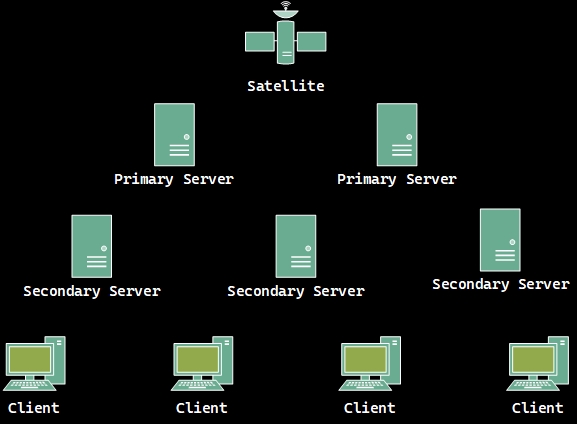
How can this protocol be applied at large scale? There are over 2 billion computers in the world, and only a tiny fraction of them are equipped with atomic clocks, out of which an even tinier fraction are being used as NTP servers. In order to not flood these few machines with requests, there are multiple layers of servers that maintain the current time. The ones in the first layer, called primary servers, receive the timestamp from an authoritative clock source, such as an atomic clock or a GPS signal. All other layers, composed of secondary servers, maintain their clock by communicating with multiple servers from the layer above, through NTP. In the end, clients can reliably obtain the current time from the servers in the last layer.

In practice

NTP Pool Project and Google Public NTP are two examples of reliable NTP services. The former is being used by hundreds of millions of systems around the world, and it’s the default “time-server” for most major Linux distributions.
On a Linux machine, the system time and date are controlled through timedatectl. Simply typing the command provides the current status of the system clock, including whether network time synchronization is active. For a more compact, machine-readable output, run timedatectl show.

Timezone=Europe/Bucharest
LocalRTC=no
CanNTP=yes
NTP=yes
NTPSynchronized=yes
TimeUSec=Sat 2023-01-21 00:27:51 EET
RTCTimeUSec=Sat 2023-01-21 00:27:52 EET

Network time synchronization can be enabled using timedatectl set-ntp 1. To set the time and date from a Google NTP server, you can run sudo ntpdate time.google.com. Feel free to fetch the time programmatically from any of these NTP services and play around with it.

from ntplib import NTPClient
from datetime import datetime

client = NTPClient()
response = client.request('time.google.com')

t1 = response.orig_time
t2 = response.recv_time
t3 = response.tx_time
t4 = response.dest_time
delta = (t4 - t1) - (t3 - t2)
theta = t3 + delta / 2 - t4
current_clock = datetime.now()
adjusted_clock = datetime.fromtimestamp(datetime.timestamp(current_clock) + theta)

print(f't1={t1}')
print(f't2={t2}')
print(f't3={t3}')
print(f't1={t4}')
print(f'delta={delta}')
print(f'theta={theta}')
print(f'Current Clock: {current_clock}')
print(f'NTP Adjusted Clock: {adjusted_clock}')

The Berkeley algorithm

Sometimes, the real atomic time does not matter. For example, in a system that’s not connected to the internet, this would be rather impractical to fetch. For many purposes, it is sufficient that all machines agree on the same time. The basic idea of this internal clock synchronization algorithm is to configure a time daemon that polls every machine periodically and ask what time it is there. Based on the answers, it computes the average time and tells all the other machines to adjust their clock accordingly. After the time daemon is initialized, the goal is to get everyone to happily agree on a current time, being that UTC or not.

Monotonic clocks

Real-time clocks, such as the system time displayed by the date command, can be subject to various adjustments, as we’ve seen, due to NTP. When trying to get a good measurement of the time difference between events that happened on the same machine, such as capturing the execution time of a function, monotonic clocks are much better suited than real-time clocks. These clocks offer higher resolution (possibly nanoseconds) and are not affected by NTP. Their timestamp would not make sense across different machines, as it’s not relative to a predefined date and can be reset when the computer reboots, but they keep track of the time elapsed, from the perspective of the local machine, and most importantly, their value is only ever-increasing (hence the name monotonic). Every OS has some way of tracking monotonic time, and programming languages usually provide some abstraction over that. In C++, std::chrono::steady_clock can be used for measuring such time intervals, at high precision. The following example illustrates how the execution time of an arbitrary lambda function could be measured using a monotonic clock.

#include <chrono>

auto get_exec_time(auto&& lambda) {
    using namespace std::chrono;
    steady_clock::time_point start = steady_clock::now();
    lambda();
    steady_clock::time_point end = steady_clock::now();
    return duration_cast<nanoseconds>(end - start).count();
}

Stating the problem

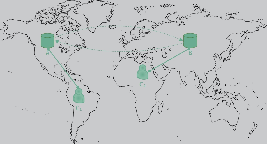
Often enough, in a database system, updates made to one database instance are automatically propagated to other instances, called replicas. This process is called replication, and its purpose is to improve data availability, increase scalability and provide better disaster recovery capabilities. For the sake of simplicity, consider a database cluster composed of just two servers, A and B, located in different corners of the world. While both A and B can be accessed by clients and are able to receive updates at all times, they have to be kept in sync, meaning that they should store the exact same copies of the data. In order to improve the overall response time of the system, a query is always forwarded to the nearest replica. This optimization does not come without a cost, because now each update operation has to be carried out at two replicas.

Assume that both replicas are perfectly in sync and contain the following document:

{
  doc: "foo",
  value: 42
}

At some point, two different clients (we’ll identify them as C₁ and C₂) try to update the document’s value, each using a different query, as expressed below in AQL syntax:

C₁ tries to add 1

FOR doc IN bar
    FILTER doc.name == "foo"
    UPDATE doc WITH {
        value: doc.value + 1
    } IN bar

C₂ tries to multiply by 2

FOR doc IN bar
    FILTER doc.name == "foo"
    UPDATE doc WITH {
        value: doc.value * 2
    } IN bar

Each server applies the query it receives and immediately sends the update to all other replicas. In case of A, C₁‘s update is performed before C₂‘s update. In contrast, the database at B will apply C₂‘s update before C₁‘s. Consequently, the database at A will record {doc: "foo", value: 86}, whereas the one at B records {doc: "foo", value: 85}. The problem that we are faced with is that the two update operations should have been performed in the same order at each copy. Although it makes a difference whether the addition is applied before the multiplication or the other way around, which order is followed is not important from a consistency point of view. The important issue is that both copies should be exactly the same.

Preconditions

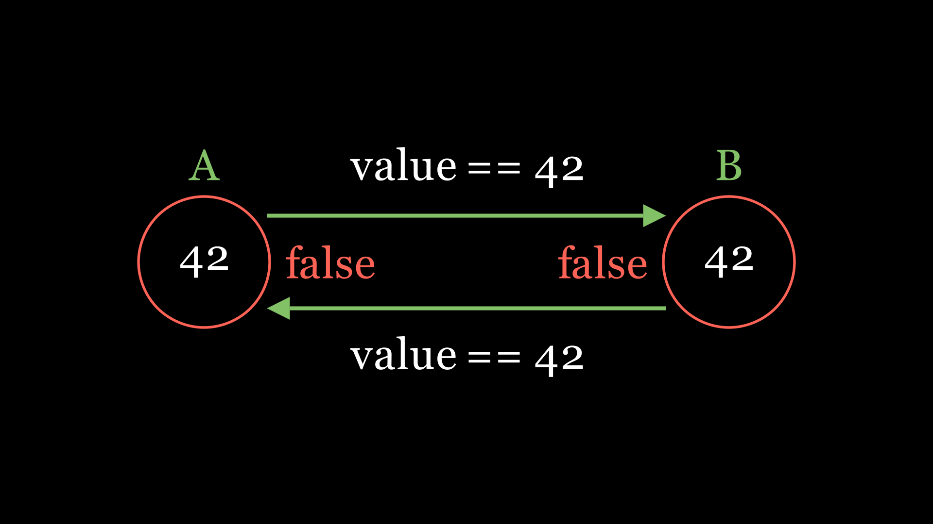
Let me start by discussing the most basic approach (in my opinion), at least in terms of implementation. Instead of passing raw updates between replicas, we could choose to always send the fully updated document instead. This doesn’t fix the problem immediately, because A could end up with 43 and pass that to B, while, in contrast, B applies 84 and passes it to A. The replicas would just confuse one another and get out of sync. What we need is more coordination between them. Upon receiving an update, a server (we can call it the sender) does not apply it immediately. Instead, it asks all other servers if they can accept the update, by passing a precondition to them. A precondition is a condition that must be true before a particular operation can be executed. In our case, the precondition is that the current value of the document is 42. If this check succeeds, it means that both the sender and the replica have the same copy of the document. Only after all replicas checked true for the precondition, the sender can apply the update itself and instruct the others to do the same. However, if the precondition fails for any of the replicas, the sender has to abort the query and return an error to the client.

What happens when A and B both receive different queries and each sends a precondition at the same time? This situation can give rise to a write-write conflict. While trying to update the same key, both send the same precondition to each other, which succeeds, since both still hold the initial value of the document. Upon receiving confirmation, they apply the update locally and send the new version of the value to each other. We need to make sure a server never replies true on a precondition referring to a key that it is trying to change itself. This acts as a global lock on the key, rejecting any attempts to update it concurrently.

Note that this approach does not scale well. Having a global lock can become frustrating for clients, as their usual approach is to retry the query in case of failure. The more replicas the system has, the longer it will take to synchronize them, which only causes the lock to be held for longer periods of time. The more clients there are, as they try to modify the same key, the easier it is for them to block each other with every retry.
Previously, we stated that a server needs confirmation from all other replicas, before executing a query. If one of them fails, the entire cluster gets blocked in read-only mode until the situation gets fixed. This is a huge disadvantage.
Nevertheless, in practice, preconditions are quite useful when a client wants to make sure the update it sends will have the desired effect. In other words, assuming the database cluster takes care of replication, the client might want to update a document, but only if that document had not changed in the meantime. This way, the client sends its current value or hash of the document together with the new value, and the cluster applies the update only if its document matches the one sent by the client. This is similar to a compare_exchange operation in C++.

Timestamps

Going back to the core problem, what we really want is that all updates are performed by all replicas in the same order. Is it possible to achieve this by passing physical timestamps along with the update operations? In this approach, each message is always timestamped with the current time of its sender, obtained from a physical clock. Let’s simplify the discussion, by assuming that no messages are lost and that messages from the same sender are received in the same order they were sent. This is a big assumption, but it allows us to truly focus on the ordering problem.
When a node receives a message, it is put into a local queue, ordered according to its timestamp. The receiver broadcasts (sends a message to all other nodes) an acknowledgment. A node can deliver a queued message to the application it is running only when that message is at the head of the queue and has been acknowledged by each other node.
Consider the same scenario as in the example above, involving two nodes, A and B. A sends message m₁, which according to A’s clock, occurs at t₁. On the other side, B prepares to send message m₂, timestamped with t₂. Assuming t₁ < t₂, after A and B receive each other’s messages, their queues will contain [m₁, m₂] exactly in this order. Regardless of the order in which acknowledgments arrive, m₁ is going to be passed to the underlying application before m₂, on both nodes. This ensures all nodes agree on a single, coherent view of the shared data, providing consistency. However, this approach has a major drawback: it is based on the assumption that all nodes have their physical clocks synchronized. What if A’s clock is 1 minute ahead of B’s? For every message sent by A, B has 60 seconds to send as many messages as it wants, during which its messages will take priority over A’s, since B’s timestamps are always lower. Apart from the fact that physical clocks may be subject to sudden change, clock drift (which is impossible to avoid on the long run), can cause scalability issues. The following animation illustrates how this kind of unfairness between the two example nodes, A and B, can occur. Even though A is the first to send its message, B’s messages are queued first.

The values of the timestamps do not matter in relation to UTC, it’s just that the clocks have to be synchronized. This is where the Berkeley algorithm could be put to good use. The downside of that is, the time daemon may become a single point of failure in the system.

Google TrueTime

Turns out, given enough resources, it is actually possible to use physical timestamps in practice. Although infinite precision is asking too much, we can come pretty close. TrueTime is Google’s solution to providing globally consistent timestamps, designed for their Spanner database. Back in 2006, when Google was using MySQL at massive scale, the process of re-sharding a cluster took them about two years. That’s how Spanner was born, designed to fit Google’s needs for scalability. TrueTime represents each timestamp as an interval [T_earliest, T_latest]. The service essentially provides three operations:

Operation	Result
TT.now()	time interval [Tearliest, Tlatest]
TT.after(t)	true if timestamp t has definitely passed
TT.before(t)	true if timestamp t has definitely not arrived

The most important aspect is that T_earliest and T_latest are guaranteed bounds. However, if the difference between them would be 60 seconds, we could end up with the same scalability issues as above. Remarkably, the engineers at Google have reduced it to just 6ms. To achieve that, several time-master machines, equipped with accurate GPS receivers or atomic clocks, are installed in each data center. All running nodes regularly poll a variety of masters and apply statistical filters to reject outliers and promote the best candidate time. Meanwhile, the performance of the system is continuously monitored and “bad” machines are removed. In this way, Spanner synchronizes and maintains the same time across all nodes globally spread across multiple data centers.
There’s lots of cool things to discuss about Google Spanner. It was the first system to distribute data at global scale and support externally-consistent distributed transactions. In simpler terms, it ensures that transactions occurring on different systems appear as if they were executed in a single, global order to external observers. Achieving externally consistent distributed transactions is no easy feat, as it typically involves coordination protocols, such as two-phase commit (2PC), and timestamp ordering mechanisms. To learn more about the inner workings of Google Spanner, check out the original paper.

Logical Clocks

Not everyone has the resources to build a system like TrueTime. Luckily, there are simpler ways to reason about the ordering of events in a cluster. Leslie Lamport pointed out that nodes don’t have to agree on what time it is, but rather on the order in which events occur, and these are two different problems. Previously, when we discussed the naive approach of using physical timestamps, we actually came pretty close to logical clocks. It’s only that, for the physical ones, we use an external device to increment it, while logical clocks are incremented with the occurrence of every event. An event is something happening at one node: sending or receiving a message, or a local execution step.

Ordering events

Before we can discuss how logical clocks work, we need to understand the criteria on which events may be ordered. We won’t be relying on physical clocks, but rather on the relation between different events. What does it mean for an event A to happen before another event B? Are we able to tell that an event was caused by another?

Causality

In one of his lectures, Dr. Martin Kleppmann beautifully defined the concepts presented here. Causality considers whether information could have flowed from one event to another, and thus whether one event may have influenced another. Given two events, A and B, when can we say that A causes (or influences) B?

• When A happens before B, we can say A might have caused B
• When A and B are concurrent, we can say that A cannot have caused B

Although this is probably not what one would expect from the description of causality, essentially, it allows us to rule out the existence of causality between two events. However, we cannot confirm it.

Happens-before relation

In his Time, Clocks, and the Ordering of Events in a Distributed System paper, Lamport introduced the happens-before relation, which essentially defines partial ordering of events in a distributed system. He made some fundamental observations on top of which Lamport Clocks can be built.
Given two events, A and B, can we check that A happened before B (noted A → B)? A happens before B means that all nodes agree that first event A occurs, then afterward, even B occurs. Unlike with the relation of causality, there’s a few ways to confirm this one for sure.

1. If the events occurred on the same node, we could use a monotonic clock to compare their times of occurrence. For example, the event of the web browser being started on your machine has clearly occurred before you have accessed this website.
2. If A is the sending of some message and B is the receipt of it, then A must-have occurred before B, because a message cannot be received unless it is sent in the first place. This one is fairly simple. Your web browser first sends a request to the server hosting this website, and only then the server is able to receive and process it.
3. If there’s another event C such that A happens before C and C happens before B, then A happens before B. Using the mathematical notation, from A → C and C → B, we can infer that A → B. Following along on the example above, the web browser is first started - that’s event A. Then, in order to access this website, a request is made to the host, that’s B. Event C occurs when the host receives the request. The event of starting the web browser must’ve happened before the host of this website received the request.

Note that this is a partial order relation. Not all elements in a partially ordered set need to be directly comparable, which distinguishes it from total order.

Concurrent events

When reasoning about the order of two events, A and B, we may arrive at one of the following conclusions:

1. A happens before B: A → B
2. B happens before A: B → A
3. None of the above, which means that A and B are concurrent: A || B

Looking back at how we defined causality, two concurrent events are independent; they could not have caused each other.

Lamport clocks

Each node assigns a (logical) timestamp T to every event. Lamport clocks are, in fact, event counters. These timestamps have the property that if event A happens before event B, then T_A < T_B. The “clock” on each node can be a simple software counter, incremented every time a new event occurs. The value by which the counter is incremented is not relevant and can even differ per node, what really matters is that it always goes forward.
Consider three nodes, A, B and C, each having its clock incremented by 6, 8 and 10 units respectively. At time 6, node A sends message m₁ to node B. When this message arrives, the logical clock in node B is incremented and reads 16. At time 60, C sends m₃ to B. Although it leaves the node at time 60, it arrives at time 56, according to B’s clock. Following the happens-before relation, since m₃ left at 60, it must arrive at 61 or later. Therefore, each message carries a sending time according to the sender’s clock. When a message arrives and the receiver’s clocks shows a value prior to the time the message was sent, the receiver fast-forwards its clock to be one more than the sending time, since the act of sending the message happens before receiving it. In practice, it is usually required that no two events happen at the same time, in other words, each logical timestamp must be unique. To address this problem, we could use tuples containing the node’s unique identifier and its logical counter value. For example, if we have two events (61, A) and (61, B), then (61, A) < (61, B).

As for the implementation, the logical clock lives in the middleware layer, between the application network layers. The counter on each node is initialized to 0. Then, the algorithm is as follows:

1. Before executing an internal event, a node increments its counter by 1.
2. Before sending a message, a node increments its counter first, so all previously occurring events have a lower timestamp. The message’s timestamp is set to the incremented counter value and the message is sent over the network.
3. Upon receiving a message, a node first adjusts its local counter to be the maximum between its current value and the timestamp of the message. After that, the counter is incremented, in order to establish a happens-before relation between the sending and the receipt.

class Node:
    def __init__(self):
        self.counter = 0

    def execute_event(e: Event):
        self.counter += 1
        e.execute()
    
    def send_message(m: Message):
        self.counter += 1
        m.timestamp = counter
        m.send()
    
    def receive_message(m: Message):
        self.counter = max(counter, m.timestamp)
        self.counter += 1

When a node receives a message, it is put into a local queue (a priority queue, to be more precise), ordered according to its (id, timestamp) tuple. The receiver broadcasts an acknowledgment to the other nodes. A node can deliver a queued message to the application layer only when that message is at the head of the queue, and it has received an acknowledgment from all other nodes. The nodes eventually iterate through the same copy of the local queue, which means that all messages are delivered in the same order everywhere.
Click the Play button below for a live simulation of Lamport Clocks, or interact with the “servers” yourself, by clicking exec or send on each circle. Use the slider to control the animation speed.

Broadcasting

In order to keep things simple, the above explanation was based on two assumptions:

• The network is reliable, meaning that messages are never lost.
• The network is ordered, meaning that messages are delivered in the same order they were sent.

In reality, these assumptions are not always true.

Reliable broadcast

When a node wants to broadcast a message, it individually sends that message to every other node in the cluster. However, it could happen that a message is dropped, and the sender crashes before retransmitting it. In this case, some nodes never get the message. We can enlist the help of the other nodes to make the system more reliable. The first time a node receives a message, it forwards it to everyone else. This way, if some nodes crash, all the remaining ones are guaranteed to receive every message. Unfortunately, this approach comes with a whopping O(n²) complexity, as each node will receive every message n - 1 times. For a small distributed system, this is not a problem, but for a large one, this is a huge overhead.
We can choose to sacrifice some reliability in favor of efficiency. The protocol can be tweaked such that when a node wishes to broadcast a message, it sends it only to a subset of nodes, chosen at random. Likewise, on receiving a message for the first time, a node forwards it to fixed number of random nodes. This is called a gossip protocol, and in practice, if the parameters of the algorithm are chosen carefully, the probability of a message being lost can be very small. Notice how similar this looks to a breadth-first search in a graph.

Total order broadcast

If we attach a Lamport timestamp to every message, each node maintains a priority queue and delivers the messages in the total order of their timestamp. The question is, when a node receives a message with timestamp T, how does it know if it has seen all messages with timestamp less than T? As the timestamp can be increased by an arbitrary amount, due to local events on each node, there is no way of telling whether some messages are missing, or there’s been a burst of local events. What we want is a guarantee that messages sent by the same node are delivered in the same order they were sent. This includes a node’s deliveries to itself, as its own messages are also part of the priority queue.
The solution is to keep a vector (could also be a map) of size N at each node, where N is the number of nodes in the cluster. Each element of the vector is a counter, representing the number of messages delivered by a particular node. Also, nodes maintain a counter of the number of messages they sent themselves. A node holds back a message until it receives the next message in sequence from the same sender. Only then, it considers delivering the previous message to the application and increments the counter corresponding to the sender. This approach is called FIFO broadcast, and combined with Lamport timestamps and reliable broadcasting, it establishes total order broadcasting.

class Node:
    def __init__(self):
        self.id = generate_id()
        self.counter = 0  # Lamport clock
        self.vector = [0] * N  # vector[i] is the number of messages delivered from node i
        self.sent = 0  # number of messages sent by this node
        self.queue = PriorityQueue()

    def execute_event(e: Event):
        self.counter += 1
        e.execute()
    
    def send_message(m: Message):
        # conceptually, the node also sends the message to itself
        self.counter += 1
        self.sent += 1
        m.timestamp = counter
        m.sent = sent  # the message carries the number of messages sent by this node so far
        m.sender_id = self.id
        m.send()
    
    def receive_message(m: Message):
        # adjust the logical clock
        self.counter = max(counter, m.timestamp[0])
        self.counter += 1
        
        self.queue.append(m)
        top = self.queue[0]
        
        if (not is_ack(top)):
            # don't do anything unless the message has been acknowledged by all nodes
            return
        
        if (top.sent == self.vector[top.sender_id] + 1):
            # this is indeed the next message to be delivered from that sender
            self.queue.pop()
            top.deliver()
            self.vector[top.sender_id] += 1

You may have noticed that the code above is missing some details, such as the PriorityQueue implementation. It is only meant to illustrate the idea behind broadcasting. However, I would like to touch upon the is_ack function, as it deserves a paragraph of its own. A simple way to implement acknowledgements is to have each node broadcast an acknowledgement for every message it receives, containing the ID of the message it wants to acknowledge. This way, for every message in the queue, a node maintains a counter, msg.ack_count, which gets incremented every time it receives an acknowledgement for that message. A message is fully acknowledged when msg.ack_count == N. Note that sending an explicit acknowledgement message is not necessary. As every node broadcasts each message to all other nodes, the broadcast itself could serve as an acknowledgement, since it’s a clear indication that the node has received the message, otherwise it would not have broadcast it.
I also wrote a complete implementation of the above algorithm, which you can find here.

Practical considerations

Total order broadcasting is an important vehicle for replicated services, where the replicas are kept consistent by letting them execute the same operations in the same order everywhere. As the replicas essentially follow the same transitions in the same finite state machine, it is also known as state machine replication.
The approach described above is not fault-tolerant: the crash of a single node can stop all other nodes from being able to deliver messages. If a node crashes or is partitioned from the rest of the cluster, the other nodes need a way to detect that, in order to recover. We can achieve this by making the nodes periodically send heartbeat messages to each other. If a node doesn’t receive heartbeats from another node for a long time, it can assume that the other node has crashed. In that case, all messages which came from it can be discarded, thus unblocking the queue, and the node can be removed from the cluster. When a node comes back online and notices that it is not part of the cluster, it rejoins the cluster as a “fresh” node and obtains a snapshot of the current state from the other nodes (easier said than done).
Often times, a particular node is designated as leader. To broadcast a message, a node has to send it to the leader, which then forwards it to all other nodes via FIFO broadcast. However, we are faced with the same problem as before: if the leader crashes, no more messages can be delivered. Eventually, the other nodes can detect that the leader is no longer available, but changing the leader safely is not trivial. In order for this article not to become exceedingly complex, we won’t go into that rabbit hole. Just be aware that in this article we discuss leaderless algorithms, but other approaches exist.

Vector clocks

Going back to the happens-before relation, recall that Lamport clocks have the following property: if A happens before B, then A has a smaller timestamp than B. However, the converse is not true: if A has a smaller timestamp than B, it doesn’t necessarily mean that A happened before B. In other words, we cannot use Lamport timestamps to determine causality between events, since in order to do that, we would need to infer the happens-before relation from the timestamps. We are looking for a different algorithm, one that can yield causality information from timestamps.
The idea behind vector clocks is very similar to the one behind Lamport clocks. In a way, vector clocks are just an extension of Lamport clocks. Instead of having a single counter, each node has a vector of counters, one for each node in the cluster. When a node sends a message, it increments its own counter and copies the vector of counters from its local state. When a node receives a message, it increments its own counter and updates its vector of counters by taking the maximum value between its own vector and the vector in the received message. To formalize this a bit, the vector clock at each node has the following properties:

• V_i[i] is the number of events that have occurred so far at node i, sort of like its own logical clock
• V_i[j], for every j different from i, is the number of events that have occurred so far at node j as seen by node i, in other words, it is i’s knowledge of the local time at j

class Node:
    def __init__(self, idx):
        self.index = idx  # the index of this node in the cluster
        self.vector = [0] * N  # all counters are initialized to 0

    def execute_event(e: Event):
        self.vector[self.index] += 1
        e.execute()
    
    def send_message(m: Message):
        self.vector[self.index] += 1
        m.timestamp = self.vector  # send the entire vector together with the message
        m.send()
    
    def receive_message(m: Message):
        for idx in range(N):
            self.vector[idx] = max(self.vector[idx], m.timestamp[idx])
        self.vector[self.index] += 1

By examining two vector clocks, we can derive their causal order - whether one happened before the other or they are concurrent. If timestamp t₁ is smaller than timestamp t₂, then t₁ happened before t₂. We say a vector is smaller than another if all its components compare less than or equal to the corresponding components of the other vector, and there is at least one component that is strictly less than its corresponding component of the other vector. In Python, the condition could be written as all(t1[i] <= t2[i] for i in range(N)) and any(t1[i] < t2[i] for i in range(N)).
To give some examples, consider the following vector clocks:

• Happens-before: (2, 1, 0) -> (3, 3, 2)
• Concurrent: (2, 3, 2) || (1, 2, 4)

Below is an animation of the vector clock algorithm in action. At the end, you’ll find an image showing all transitions from a different perspective.

Needless to say, the causality relation that can be derived from vector clocks is purely theoretical. In practice, without knowing the actual information contained in messages, it is not possible to state with certainty that there is indeed a causal relation.

Causal broadcast

Using vector clocks, it is possible to ensure that a message is delivered to the application only if all messages that causally precede it have been delivered as well. Hence, we say the messages are delivered in causal order. The algorithm is similar to the one used for FIFO broadcast. The vectors themselves contain the same information: V[i] is the number of messages that have been delivered to the application, sent from node i. When a node wants to broadcast a message, it attaches a copy of its own vector clock to that message, adjusting with an increment the counter at its corresponding index, thus ensuring that each message broadcast by this node has a causal dependency on the previous message broadcast by the same node. Upon receiving a message, the node adds it to a queue, only updating its internal clock when messages are delivered to the application. Keep in mind that the vector elements don’t count events, but rather the number of messages that have been delivered from each sender.
Suppose V is the vector clock at A. In order for node A to deliver a message m with timestamp t, sent by node B, the following conditions must be met:

• t[B] = V[B] + 1, meaning that m is the next message that A expects from B. This is the same condition as for FIFO total order broadcast.
• t[i] <= V[i], for every i different from B. This means that A has already delivered all messages that B has delivered before it sent m. This is what differentiates causal broadcast from FIFO total order broadcast. This condition ensures that all messages that may have caused m are delivered before m.

class Node:
    def __init__(self, idx):
        self.index = idx  #  the index of this node in the cluster
        self.vector = [0] * N  # all counters are initialized to 0
        self.sent = 0  #  the number of messages sent so far by this node
        self.queue = []  # the queue of messages received but not yet delivered

    def send_message(m: Message):
        m.timestamp = self.vector.copy()  # send the entire vector together with the message
        m.timestamp[self.index] = self.sent + 1
        m.index = self.index
        m.send()
        self.sent += 1
    
    def should_deliver(m: Message):
        t = m.timestamp
        condition1 = t[m.index] == self.vector[m.index] + 1
        condition2 = all(t[i] <= self.vector[i] for i in range(N) if i != m.index)
        return condition1 and condition2
    
    def receive_message(m: Message):
        self.queue.append(m)
        delivering = True
        while delivering:
            delivering = None
            for msg in self.queue:
                t = msg.timestamp
                if self.should_deliver(msg):
                    delivering = msg
                    break
            if delivering:
                self.queue.remove(delivering)
                delivering.deliver()
                self.vector = [max(self.vector[i], delivering.timestamp[i]) for i in range(N)]

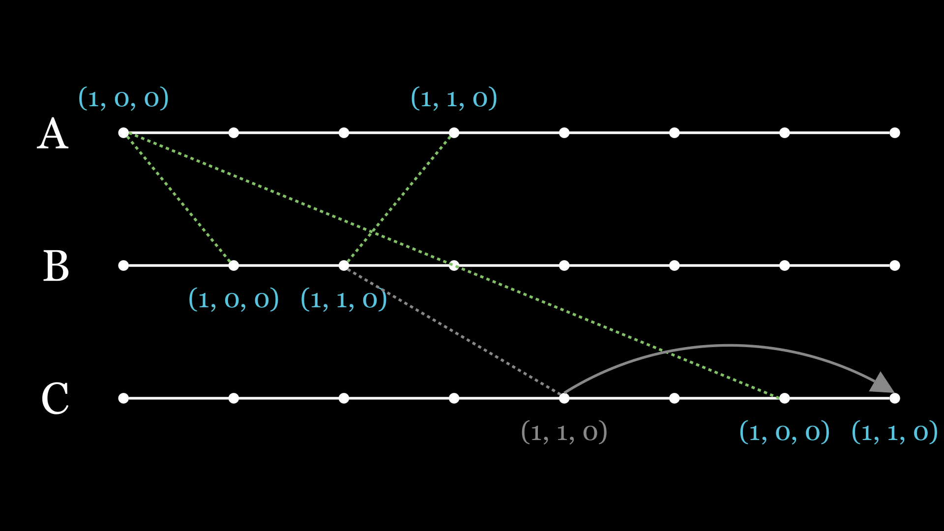
When node A sends its message with timestamp (1, 0, 0), it arrives at B after 1 second, but due to network latency, it takes 6 seconds for C to get the message. Therefore, when B sends its message with timestamp (1, 1, 0), it arrives at C ahead of (1, 0, 0). This is what the causal broadcast algorithm tries to correct. C notices that it’s missing a message from A and waits for that to be delivered first.

It is important to note that causal broadcast is weaker than total order broadcast. Specifically, if two messages are not related in any way to each other, they may be delivered in different order at different locations.

Hybrid Logical Clocks

We can combine both physical clocks and logical clocks into what’s called a hybrid logical clock. The resulting algorithm consists of two components:

• a physical component, usually synchronized to NTP, used to represent the actual wall-clock time
• a logical component, incremented whenever there are events happening whiting the same physical time

Therefore, a HLC’s timestamp is a tuple (t, c), where t is the physical time and c is the logical time. The physical component is compared first, and in case of equality, the logical component is used. HCLs preserve the properties of Lamport clocks: if A happens before B, then HLC(A) < HLC(B). As they maintain a bounded divergence from physical time, they are useful for applications that require a certain degree of real-life synchronization. One important aspect of HLCs is that they are always monotonically increasing, unlike simple physical clocks. Another great thing about them is that their implementation can be of constant space complexity, as opposed to vector clocks.

ArangoDB uses 64-bit integers to represent such hybrid timestamps, out of which 44 bits are used by the physical component and the remaining 20 bits by the logical component. A C++ implementation can be found in HybridLogicalClock.h and HybridLogicalClock.cpp. If you’re familiar with Go, you can also check out CockroachDB’s implementation. Below, I will summarize the algorithm and give a simple Python implementation inspired by the one in ArangoDB.
Whenever we want to generate a new timestamp, we first fetch the current physical time from the system. As with logical counters, we always update the clock to the maximum value encountered across nodes. If the current physical time is less than or equal to the last known physical time in our HLC instance, we keep the physical component as is and increment the logical component. Otherwise, if the current physical time is greater, we update the physical component and reset the logical component to 0. This way, we ensure that the newly generated timestamp is always greater than the last one.
Whenever we receive a timestamp from another node, we proceed to updating our own clock. For the physical component, we always take the maximum between the current system time, the last known physical time and the physical component extracted from the received message. As for the logical component, we adjust it according to which of these three options has yielded the maximum value, making sure the newly generated timestamp always goes forward.

from collections import namedtuple
from datetime import datetime


Timestamp = namedtuple('Timestamp', ['physical', 'logical'])


class HLC:
    """
    Hybrid Logical Clock
    """
    def __init__(self):
        self._last_timestamp = Timestamp(0, 0)

    @staticmethod
    def get_physical_time():
        """
        Retrieve the current physical time.
        """
        return datetime.now().timestamp()

    def get_timestamp(self):
        """
        Generate a new timestamp.
        """
        physical = self.get_physical_time()
        if physical <= self._last_timestamp.physical:
            # Physical time stays the same,
            # but the logical component gets updated.
            physical = self._last_timestamp.physical
            logical = self._last_timestamp.logical + 1
        else:
            logical = 0
        self._last_timestamp = Timestamp(physical, logical)
        return self._last_timestamp

    def get_timestamp_and_adjust(self, received: Timestamp):
        """
        Adjust the local clock based on a received timestamp and return a new timestamp.
        """
        physical = max(self.get_physical_time(),
                       self._last_timestamp.physical,
                       received.physical)
        if physical == self._last_timestamp.physical:
            if physical == received.physical:
                # The last recorded timestamp and the received timestamp
                # have the same physical time, greater than the current physical time.
                logical = max(self._last_timestamp.logical, received.logical) + 1
            else:
                # The last recorded timestamp has a higher physical time
                # than the received timestamp.
                logical = self._last_timestamp.logical + 1
        else:
            if physical == received.physical:
                # The received timestamp has a higher physical time
                # than the last recorded timestamp.
                logical = received.logical + 1
            else:
                # The current physical time is higher than
                # both the last recorded timestamp and the received timestamp.
                logical = 0
        self._last_timestamp = Timestamp(physical, logical)
        return self._last_timestamp

In practice

There are various usages for HLCs in modern databases, apart from maintaining causality across nodes. I referred to ArangoDB multiple times in this article, but other databases make use of them as well. For example, CockroachDB relies on them in order to provide their transactional isolation guarantees. Another example is MongoDB, using them in their MVCC storage implementation. MVCC is a database technique that allows multiple transactions to access and modify shared data concurrently without conflicts.

Closing thoughts

We discussed various ways in which time is represented in distributed systems and what are their challenges. In the end, I would like to leave you with the words of Anthony G. Oettinger:

Time flies like an arrow; fruit flies like a banana.

References and Further Reading

• M. van Steen and A.S. Tanenbaum, Distributed Systems, 3rd ed., distributed-systems.net, 2017.
• tldp.org
• chelseaclock.com
• wikipedia.org/wiki/Quartz_clock
• Distributed Systems Lectures by Dr Martin Kleppmann
• pngwing.com
• APNIC
• news.ucr.edu
• Kevin Sookocheff
• Internals of Google Cloud Spanner
• All Things Clock, Time and Order in Distributed Systems
• Cockroach Labs